🍁 Autoregressive Models date 13.09.2022
Motivation, Key Ideas by Hidir Yesiltepe

🍁 Introduction
Autoregressive models are a sequential deep generative models which are among the constituent part of the state-of-the art models in different domains such as Image Generation, Audio Generation , Gesture Generation and Large Language Models.
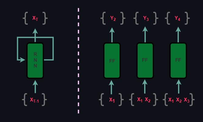
Since autoregressive models are sequential, they are similar to RNNs but they differ in the method. While RNNs are recurrent, autoregressive models are feed-forward yet both methods are supervised.
On the other hand, because autoregressive models are a type of generative models, their expressiveness capability is often compared against VAEs and GANs but there are some core differences. First of all, although autoregressive models and VAEs are explicit models, due to intractable likelihood computation, VAEs optimize Evidence Lower Bound whereas in autoregressive models likelihood is optimized directly. When it comes to comparing autoregressive models with GANs, GANs are implicit models which optimizes minimax objective as opposed to explicit likelihood based autoregressive models.
| Model | Main Objective | Explicit/Implicit | |
|---|---|---|---|
| 0 | Autoregressive Models | Log-Likelihood | Explicit |
| 1 | Variational Autoencoders (VAEs) | Evidence Lower Bound (ELBO) | Explicit |
| 2 | Generative Adversarial Networks (GANs) | Minimax | Implicit |
🍁 Chain Rule
We start our discussion on autoregressive models with the chain rule of probability. From now on, we assume that we have an access to a dataset of N dimensional binary datapoints and the cardinality of M:
$$ \mathcal{D} = \{x_i\}_{i=1}^{\mathcal{M}} \hspace{60px} x_i \in R^{\mathcal{N}} \tag{1}$$
The chain rule of probability states that joint probability distribution can be factorized into conditional probability distributions. This fact constitutes the backbone of Bayesian Networks and Autoregressive Models.
$$ P(x_i) = P(x_1, ..., x_N) = P(x_1)\prod_{j=2}^{\mathcal{N}} P(x_j | x_1, ..., x_{j-1}) \tag{2} $$
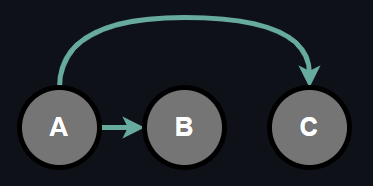
which means the probability of any random variable in the set is conditionally dependent on all the random variables preceding it and further, the dependence order is predefined and fixed. Such a dependence relationship can be graphically described as:
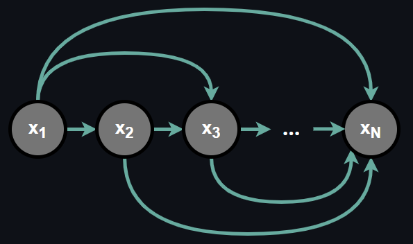
Chain rule of probability is a useful factorization because often dealing with conditional probabilities is more convenient than dealing with joint probability at once. Now the question is how can we represent such a dependence relationship?
🍁 Representation
We can represent the Equation [2] in several modelling approaches with a trade-off between expressiveness and the complexity of the models. Further in this section, we will experience that complexity of the models creates an immense limitation such that at the end we will have to make some modelling assumptions.
🍁 Tabular Representation
We can represent the conditional probabilities with a tabular form which is called Conditional Probability Table (CPT). Representing conditional probabilities in a tabular form means that for each conditional probability there is a CPT such that every configuration of random variables involving in the conditional probability have a corresponding likelihood. For the sake of visualizing, suppose we have 3 binary random variables.
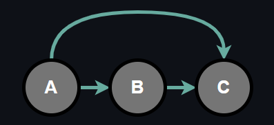
The joint probability of random variables can be factorized into conditional probabilities by chain rule as follows:
$$ P(A, B, C) = P(A)P(B|A)P(C|A, B) \tag{3}$$
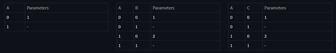
As a result of this factorization, corresponding CPTs can be viewed as following tables:
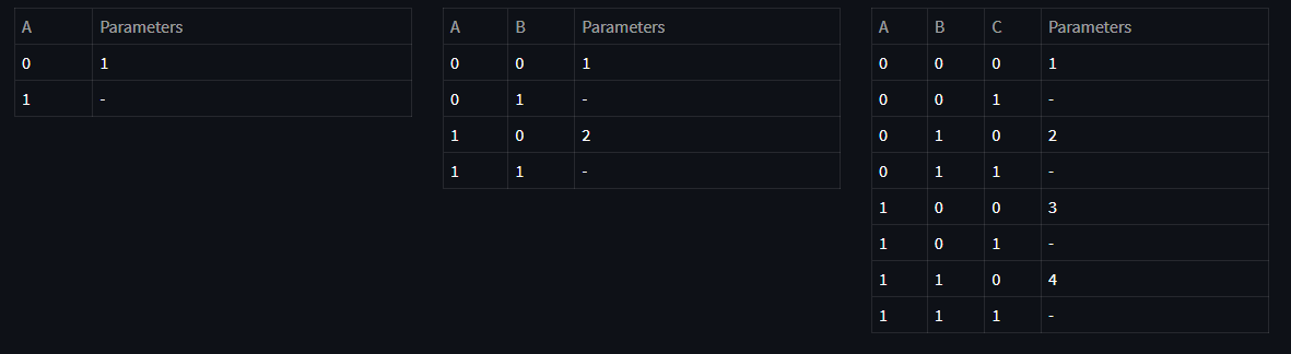
Above, you see the CPT tables representing each conditional probability along with minimum number of parameters required to represent each table. For example, since for random variable A we have:
$$ P(A = 0) = 1 - P(A=1) \tag{4} $$
we don't have to use two variables here, only one variable can represent the entire table. Same applies for others by grouping the conditioning variables. Now, let's see the advantages and disadvantages of tabular representation.
The advantage of tabular modelling choice is that we can represent any joint distribution exactly which means that among the other modelling choices, tabular form representation have the highest expressiveness. But it turns out that to be able to represent joint distribution in a tabular form we need exponential size parameters!
$$ P(x_1) : 2^0 \text{ parameters} $$
$$ P(x_2|x_1) : 2^1 \text{ parameters} $$
$$ P(x_3|x_1, x_2) : 2^2 \text{ parameters} $$
$$ ... $$
$$ P(x_N|x_1, ..., x_{N-1}) : 2^{N-1} \text{ parameters} $$
By geometric sum formula, we have:
$$ 2^0 + 2^1 + 2^2 + \text{ ... } + 2^{N-1} = \frac{1 - 2^N}{1 - 2} = 2^N - 1 \text{ total parameters} \tag{5} $$
To better understand what exactly exponential size parameters mean, let's give a concrete example. Binarized MNIST dataset consists of 28 x 28 images which means each data point (image) in the dataset lies in 784 dimensional space.
$$ x_i \in \{0, 1\}^{784} $$
To represent any possible joint probability in a tabular form as we described above, we would need:
$$ 2^{784} \approx 10^{236} $$
probabilities to estimate which is obviously not tractable. Observe that, current representation does not have any independence assumption, each random variable is conditionally dependent all the preceding random variables. An improvement on the parameter size would be introducing conditional independence assumptions in which our next representation exactly does.
🍁 Bayes Network
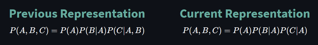
The previous approach to represent joint probability with individiual conditional probabilities as a result of chain rule was fully general and there was no conditional assumptions. Now, let's consider the same 3 binary random variable setting again and introduce a conditional independence between B and C.
Observe that above configuration is almost same as before except that now random variables B and C are independent. Depending upon the problem at hand, this might or might not be a huge assumption. Nevertheless, we make it in order to reduce the number of parameters of the model. Note that, there is no particular reason behind we chose random variables B and C, we could have chosen some other combination to make it independent as well.
With that being said, we can now represent the joint probability in terms of conditional probabilities as:
We can again utilize from CPT represent conditional probabilities as follows:
One might adopt a modelling design such that each random variable depends only on the random variable preceding it. If we generalize this assumption over N random variables we get:
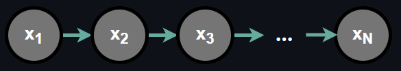
In this dependence relationship, the joint probability can be written as:
$$ P(x_1, ..., x_N) = P(x_1)\prod_{j=2}^N P(x_j|x_{j-1}) \tag{6}$$
Now let's calculate the number of parameters required to represent joint distribution in a tabular form with the assumption we have made:
$$ P(x_1) : 2^0 \text{ parameters}$$
$$ P(x_2|x_1) : 2^1 \text{ parameters}$$
$$ P(x_3|x_2) : 2^1 \text{ parameters}$$
$$ ... $$
$$ P(x_N|x_{N-1}) : 2^1 \text{ parameters}$$
As a result, in total we have:
$$ 1 + (N - 1) \times 2 = 2N - 1 \text{ total parameters}$$
It turns out that, we didn't just reduce the number of parameters drastically but also the representation capacity. Obviously a model with exponential size parameters and a model with linear size parameters does not have the same capacity. Can't we just create an expressive but yet efficient model that makes no conditional assumption?
🍁 Autoregressive Models
The main idea behind Autoregressive Models is representing the conditional distributions with Neural Networks without making any conditional independence assumption. All we need to do is parameterizing the conditional distributions with some weight vector θ.
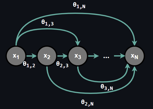
An important note here, as you can see in the figure above there is no conditional assumption in autoregressive models, all the random variables depends each and every random variable preceding it and furhter, dependence is provided by parameters θ. We can represent the joint distribution as:
$$P(x_1, ..., x_N) = P(x_1)\prod_{j=2}^N P_{Neural}(x_j| x_1, ..., x_{j-1}; θ) \tag{7}$$
In the above representation of chain rule, probabilities with Neural subscript are special functional form for conditionals. On the other hand, the very first random variable is drawn from a known distribution. It is best understood by giving a concrete example. Suppose we have an access to a Binarized Icon Dataset in which each element of the dataset is of size 7 x 7.
.png)
More explicitly, we can write the equations describing above autoregressive image generative models as following:
$$ P(x_1 = 1; θ_1) = θ_1 \hspace{80px} P(x_1 = 0; θ_1) = 1 - θ_1 \tag{8}$$
The very first random variable does not depend any other random variable so it is drawn from Bernoulli Distribution with a success parameter θ1. A significant remainder here is that P(x1 ; θ1) is not a neural network.
$$ P_{Neural}(x_2 = 1 | x_1; \theta_2) = \sigma(\theta^2_0 + \theta^2_1 \times x_1) \tag{9}$$
$$ P_{Neural}(x_3 = 1 | x_1, x_2; \theta_3) = \sigma(\theta^3_0 + \theta^3_1 \times x_1 + \theta^3_2 \times x_2) \tag{10}$$
Where sigma is a non-linear function. Often, the result of the PNeural is considered as a logit and it is represented as:
$$ P_{logit} = P_{Neural}$$
Let's attribute for what a logit is and why this result is associated with the term logit. The logit L of a probability P is defined as:
$$ L = ln\frac{P}{1-P} \tag{11}$$
which is the natural logarithm of odds. There are two important properties of logit. Firstly, the range of the logit is (-∞, ∞). Secondly, the inverse of the logit function is the sigmoid function:
$$ P = \frac{1}{1 + e^{-L}} = Sigmoid(L) \tag{12}$$
As a summary, logits are unnormalised predictions which are then normalised via softmax. Now, we know the main motivation behind autoregressive models and how a simple autoregressive model is structured. Next, we are going to take a look at the objective of autoregressive models.
🍁 Main Objective
Autoregressive models are explicit models which further means that they optimize the underlying joint distribution directly via Maximum Likelihood Estimation (MLE). Most importantly, maximizing the MLE objective is not an arbitrary choice but is a natural consequence of KL divergence between Pdata and Pmodel. In this section we will take a look at the natural relation between the KL Divergence and Maximum Likelihood Estimation.
🍁 KL & MLE Relationship
The ultimate goal of an autoregressive model is capturing the underlying probability distribution of the data. To quantify how close two distributions are we attempt to minimize the KL Divergence between the data distribution Pdata and distribution captured by an autoregressive model Pmodel:
$$ \underset{\theta}{\text{minimize}} \hspace{30px} KL(P_{data}(x) || P_{model}(x ;\theta)) \tag{13}$$
If we write the open form of KL to eliminate the terms which do not depend on parameter theta, we obtain:
$$ \underset{\theta}{\text{minimize}} \hspace{30px} \sum_x P_{data}(x) log \frac{P_{data}(x)}{P_{model}(x;\theta)} \tag{14}$$
$$ = \underset{\theta}{\text{minimize}} \hspace{30px} \sum_x P_{data}(x) log P_{data}(x) - \sum_x P_{data}(x) log P_{model}(x;\theta) \tag{15}$$
Where the first term is called the negative entropy of the random variable X and does not depend on the parameter theta. If we eliminate this term and write the second term as an expectation we obtain:
$$ = \underset{\theta}{\text{minimize}} \hspace{30px} -\mathbb{E}_{x \sim P_{data}}[log P_{model}(x;\theta)] \tag{16}$$
$$ = \underset{\theta}{\text{maximize}} \hspace{30px} \mathbb{E}_{x \sim P_{data}}[log P_{model}(x;\theta)] \tag{17}$$
As the last step, applying the Law of Large Numbers to get rid of expectation term yields:
$$ = \underset{\theta}{\text{maximize}} \hspace{30px} \underset{n \rightarrow \infty}{\text{lim}} \sum_{i=1}^n logP_{model}(x^{(i)};\theta) \tag{18}$$
$$ = \underset{\theta}{\text{maximize}} \hspace{30px} logP_{model}(x;\theta) \tag{19}$$
$$ = \underset{\theta}{\text{maximize}} \hspace{30px} P_{model}(x;\theta) \tag{20}$$
$$ = \theta_{MLE} \tag{21}$$
As the summary, since autoregressive models are likelihood based, as a consequence of minimizing the KL Divergence between the true underlying distribution and the distribution represented by the model we estimate the model parameters. It turns out that estimating the model parameters in this fashion equivalent to maximum likelihood estimation. In practice we minimize the negative log likelihood.
🍁 Inference and Sampling
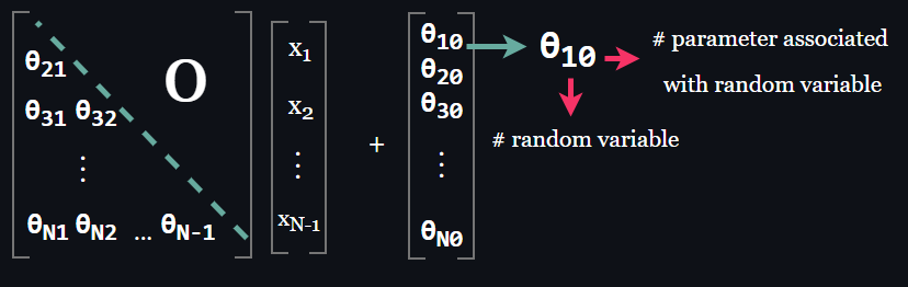
A consequence of the parameterization of the an autoregressive model is that the weight matrix is a lower triangular matrix.
$$ OR $$
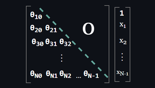
An important observation here: Inference becomes a parallel computation and fast in autoregressive models. Consider the density estimation of an arbitrary point:
$$ x = [x_1, ..., x_n]^T $$
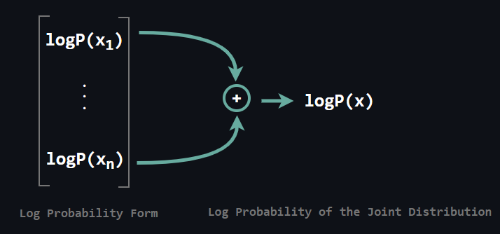
All we need to do is compute the above matrix multiplication to yield log-conditionals. Then how do we obtain log-conditionals if our architecture models logits rather than log-probabilities directly? It is quite simple as well. Compute the above matrix multiplication to yield logits, then apply softmax to yield each probability and finally apply logarithm to each probability, it is done!
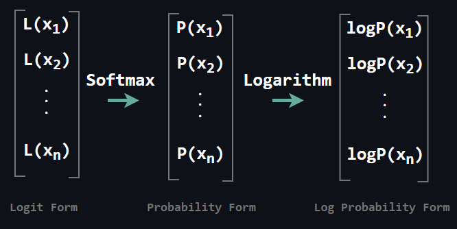
Above you see the transition in which L stands for the logit. Obtaining the objective after this step is not a big deal. It reduces to adding each conditional log probability.
Sampling on the other hand is a sequential process and slow. Why is that? Since x2 depends on x1 we need to sample x1 prior to x2. Further, since x3 depends both x1 and x2 we need to sample those prior to x3. Following this fashion brings us to a sequential process.
Our introductory discussion on Autoregressive Models ends here, hope you enjoyed! In the upcoming posts we are going to explore the prominent applications of Autoregressive Models.
🔗 Give Feedback & Ask Question!